Hi-C Data Processing

Hi-C Data Processing#

24/03/2022

Hi-C data is often used to analyze genome-wide chromatin organization, such as topologically associating domains (TADs), which are linearly contiguous regions of the genome that are associated in 3D space. Atgenomix worked with Professor Jia-Ming Chang ( external link ) of the National Chengchi University in Taiwan to develop a Hi-C data analysis pipeline on the Seqslab Platform.

In this case study, we first standardize and demonstrate a Hi-C data processing pipeline with WDL and an open-source tool HiC-Pro ( external link ). Afterwards, we then accelerate the Hi-C pipeline based on different operator pipeline configurations and finally, we show the performance evaluation.

Main WDL#

With the aide of Zhan-Wei Lin, the Hi-C data processing pipeline is standardized via WDL as shown in this HiC-Pro_0.0.6.wdl file ( external link ). Inside the main workflow, HiC-Docker, there are no subworkflows and all the tasks are called directly. In addition, in order to support multiple samples execution, a scatter operation is applied inside the main workflow.

Based on the WDL, an inputs.json file is provided as follows.

{
    "Hic_Docker.sampleName": "SRR400264_00",
    "Hic_Docker.tableFile": "/datadrive/input_files/annotation/chrom_hg19.sizes",
    "Hic_Docker.dockerImage": "atgenomix.azurecr.io/atgenomix/seqslab_runtime-1.5_ubuntu-20.04_hicpro:2021-11-08-08-00",
    "Hic_Docker.hicPath": "/HiC-Pro_3.1.0",
    "Hic_Docker.referenceGenome": "hg19",
    "Hic_Docker.bowtie2LocalOptions": "--very-sensitive -L 20 --score-min L,-0.6,-0.2 --end-to-end --reorder",
    "Hic_Docker.bowtie2GlobalOptions": "--very-sensitive -L 30 --score-min L,-0.6,-0.2 --end-to-end --reorder",
    "Hic_Docker.binSize": "20000",
    "Hic_Docker.bowtieIndexPath": "/datadrive/input_files/btw2idx/hg19",
    "Hic_Docker.bedFile": "/datadrive/input_files/annotation/HindIII_resfrag_hg19.bed",
    "Hic_Docker.nCPU": "1",
    "Hic_Docker.cutsite": "AAGCTAGCTT",
    "Hic_Docker.nMem": "100",
    "Hic_Docker.inputSamples": [["/datadrive/input_files/fastq/SRR1030718_1.fastq", "/datadrive/input_files/fastq/SRR1030718_2.fastq"]],
    "Hic_Docker.inputSettings": [["SRR400264_00", "Dixon2M"]],
    "Hic_Docker.tagR1": "_R1",
    "Hic_Docker.tagR2": "_R2",
    "Hic_Docker.resName": "Dixon2M",
    "Hic_Docker.fakeFile": "test"
}

WOM Graph#

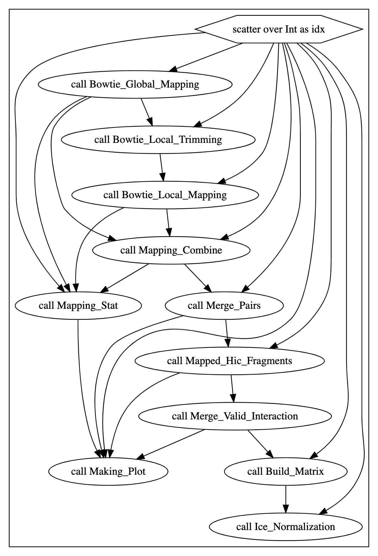
Parsed by the Cromwell womtool, we obtain the following WOM Graph which describes the Hi-C data pipeline, including tasks such as Bowtie_Global_Mapping, Bowtie_Local_Trimming, Bowtie_Local_Mapping, Mapping_Combine, Mapping_Stat, Merge_Pairs, Mapped_Hic_Fragments, Merge_Valid_Interaction, Making_Plot, Build_Matrix, and Ice_Normalization.

WOM Graph of main wdl

Parallelization Settings#

In this specific example, the FASTQ GZ files are around 6.2GB (R1) and 6.4GB (R2). By applying the following chunking settings, we can seperate these two FASTQ files into 53 partitions.

{
    "fqn": "Hic_Docker.Bowtie_Global_Mapping.sampleR1",
    "operators": {
        "format": {
            "class": "com.atgenomix.seqslab.piper.operators.format.FastqFormat"
        },
        "p_pipe": {
            "class": "com.atgenomix.seqslab.piper.operators.pipe.PPipe"
        },
        "source": {
            "class": "com.atgenomix.seqslab.piper.operators.source.FastqSource",
            "codec": "org.seqdoop.hadoop_bam.util.BGZFCodec"
        },
        "partition": {
            "class": "com.atgenomix.seqslab.piper.operators.partition.FastqPartition",
            "parallelism": "3145728"
        }
    },
    "pipelines": {
        "call": [
            "format",
            "p_pipe"
        ],
        "input": [
            "source",
            "partition",
            "format"
        ]
    }
}

Data Consistency#

In order to validate data consistency between Parallel/Non-Parallel execution, we verify the task output, Merge_Valid_Interaction, where it shows that the pair number in different categories are the same.

Statistics	Non Parallelization	Parallelization
valid_interaction	52734597	52734597
valid_interaction_rmdup	47916253	47916253
trans_interaction	10867055	10867055
cis_interaction	37049198	37049198
cis_shortRange	3556197	3556197
cis_longRange	33493001	33493001

Performance evaluation#

Based on the test results, we can see that by applying parallel settings, the execution time is largely reduced. However, the reduced execution time is not fully linear as there are some added overhead and some tasks are not fully parallizable.

It is worth mentioning that acceleration cannot be achieved by unlimitedly increasing the VM node number as you can observe that the performance with D13_v2 x 10 is very similar with D13_v2 x 20. It is because the FASTQ data is only chunked into 53 segments. In the case of D13_v2 x 10, a total of 80 CPU can be used at the same time which is already larger than the 53 segments. Therefore, allocating even more D13_v2 VM nodes is unnecessary and useless in this case.

Note

Azure D13_v2 VM has specification 8 cores CPU + 56GB RAM.